ClinReport Vignette 2: The Different Type of Statistical Tables

Get started

Start by loading all usual libraries.

library(ClinReport)
library(officer)
library(flextable)
library(dplyr)
library(reshape2)
library(nlme)
library(emmeans)
library(car)

Load your data.

# We will use fake data
data(datafake)
print(head(datafake))
#>    y_numeric y_logistic y_poisson   baseline   VAR GROUP TIMEPOINT SUBJID
#> 1 -0.4203490          1         5 -0.4203490 Cat 1     A        D0 Subj 1
#> 2 -0.1570941          1         5 -0.1570941 Cat 2     A        D0 Subj 1
#> 3         NA          0         3 -2.0853720 Cat 2     A        D0 Subj 1
#> 4 -0.4728527          0         5 -0.4728527 Cat 1     A        D0 Subj 1
#> 5 -0.8651713          1         4 -0.8651713 Cat 1     A        D0 Subj 1
#> 6 -1.5476907          1         3 -1.5476907 Cat 1     A        D0 Subj 1

Create a statistical output for a quantitative response and two explicative variables. For example a treatment group and a time variable corresponding to the visits of a clinical trial.

For that we use the report.quanti() function:

tab1=report.quanti(data=datafake,y="y_numeric",
        x1="GROUP",x2="TIMEPOINT",at.row="TIMEPOINT",
        subjid="SUBJID")

tab1
#> 
#> ############################################
#> Quantitative descriptive statistics of: y_numeric
#> ############################################
#> 
#>    TIMEPOINT Statistics      A (N=30)      B (N=21)      C (N=17)
#> 1         D0          N            30            20            16
#> 2         D0  Mean (SD)   -0.93(0.86)   -0.67(1.09)   -1.19(0.92)
#> 3         D0     Median         -0.82         -0.69         -1.26
#> 4         D0    [Q1;Q3] [-1.59;-0.16] [-1.39;-0.06] [-1.62;-0.83]
#> 5         D0  [Min;Max]  [-2.34;0.36]  [-2.44;2.10]  [-2.99;0.66]
#> 6         D0    Missing             1             1             0
#> 7                                                                
#> 8         D1          N            30            20            16
#> 9         D1  Mean (SD)    1.83(1.04)    4.17(1.28)    4.98(0.69)
#> 10        D1     Median          1.78          4.19          5.08
#> 11        D1    [Q1;Q3] [ 0.94; 2.54] [ 3.23; 4.92] [ 4.58; 5.46]
#> 12        D1  [Min;Max]  [ 0.11;3.88]  [ 1.48;6.19]  [ 3.80;6.23]
#> 13        D1    Missing             1             0             0
#> 14                                                               
#> 15        D2          N            30            20            16
#> 16        D2  Mean (SD)    1.97(1.17)    4.04(0.89)    4.90(1.36)
#> 17        D2     Median          1.66          4.19          5.06
#> 18        D2    [Q1;Q3] [ 1.23; 2.86] [ 3.62; 4.36] [ 4.34; 5.20]
#> 19        D2  [Min;Max]  [-0.18;4.36]  [ 2.03;5.63]  [ 2.39;7.96]
#> 20        D2    Missing             1             1             0
#> 21                                                               
#> 22        D3          N            30            20            16
#> 23        D3  Mean (SD)    1.78(1.17)    3.81(0.94)    5.07(1.12)
#> 24        D3     Median          1.78          3.63          5.22
#> 25        D3    [Q1;Q3] [ 0.93; 2.42] [ 3.13; 4.44] [ 4.11; 5.66]
#> 26        D3  [Min;Max]  [-0.16;3.90]  [ 2.46;6.01]  [ 3.16;7.37]
#> 27        D3    Missing             0             1             1
#> 28                                                               
#> 29        D4          N            30            20            16
#> 30        D4  Mean (SD)    1.83(0.85)    3.80(0.95)    5.17(1.03)
#> 31        D4     Median          1.67          3.83          4.88
#> 32        D4    [Q1;Q3] [ 1.26; 2.32] [ 3.12; 4.42] [ 4.69; 5.50]
#> 33        D4  [Min;Max]  [ 0.38;3.97]  [ 2.31;5.41]  [ 3.24;6.96]
#> 34        D4    Missing             1             1             1
#> 35                                                               
#> 36        D5          N            30            20            16
#> 37        D5  Mean (SD)    2.27(1.20)    3.64(1.19)    4.43(0.98)
#> 38        D5     Median          2.50          3.86          4.57
#> 39        D5    [Q1;Q3] [ 1.77; 3.21] [ 2.59; 4.60] [ 3.44; 4.97]
#> 40        D5  [Min;Max]  [-1.19;4.31]  [ 0.91;5.12]  [ 2.95;6.54]
#> 41        D5    Missing             0             0             0
#> 
#> ############################################

The at.row argument is used to space the results between each visit and the subjid argument is used to add in the columns header the total number of subjects randomized by treatment group.

Generally we want also the corresponding graphics. So you can use the specific plot function to print the corresponding graphic of your table:

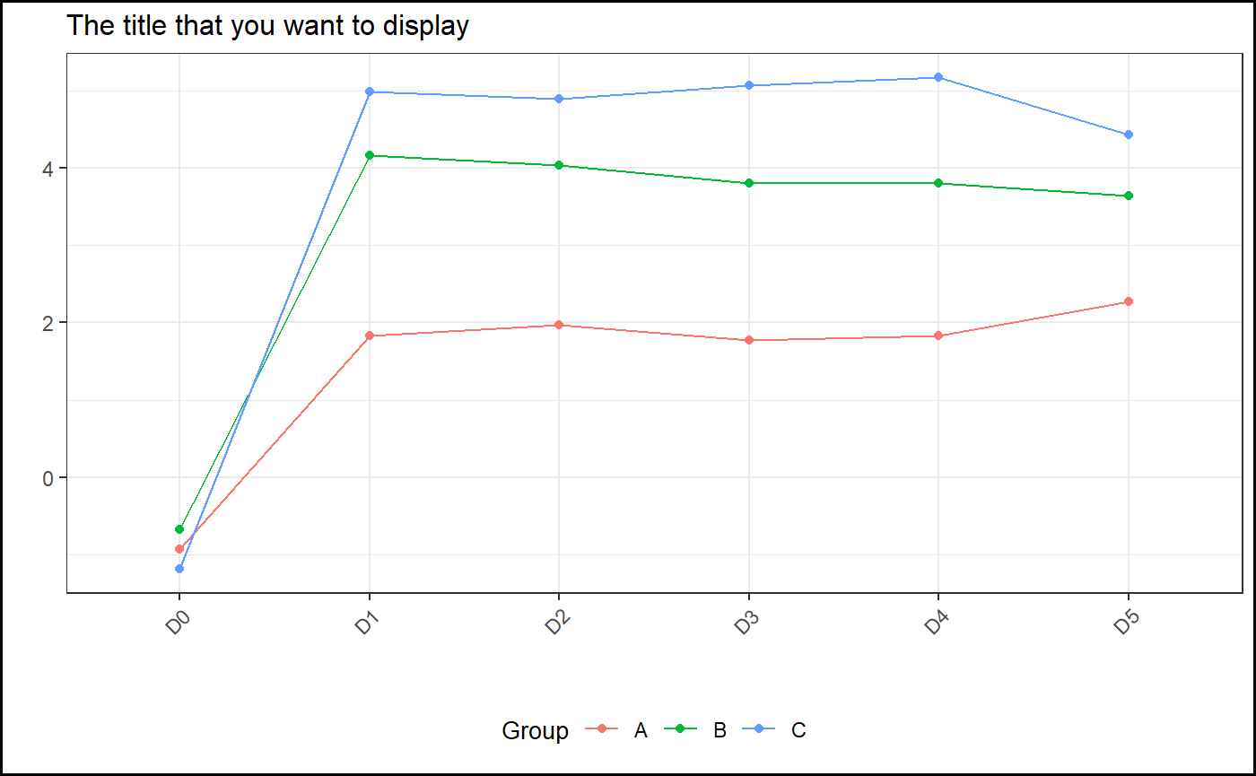
g1=plot(tab1,title="The title that you want to display")
print(g1)

You can modify the plot by using the following arguments of the plot.desc() function:

args(ClinReport:::plot.desc)
#> function (x, ..., title = "", ylim = NULL, xlim = NULL, xlab = "", 
#>     ylab = "", legend.label = "Group", add.sd = F, add.ci = F, 
#>     size.title = 10, add.line = T) 
#> NULL

Then we can use the report.doc() function which use the flextable package to format the output into a flextable object, ready to export to Microsoft Word with the officer package.

The table will look like this (we can have a preview in HTML, just to check):

report.doc(tab1,title="Quantitative statistics (2 explicative variables)",
        colspan.value="Treatment group", init.numbering =T )

Table 1: Quantitative statistics (2 explicative variables)
		Treatment group
TIMEPOINT	Statistics	A (N=30)	B (N=21)	C (N=17)
D0	N	30	20	16
	Mean (SD)	-0.93(0.86)	-0.67(1.09)	-1.19(0.92)
	Median	-0.82	-0.69	-1.26
	[Q1;Q3]	[-1.59;-0.16]	[-1.39;-0.06]	[-1.62;-0.83]
	[Min;Max]	[-2.34;0.36]	[-2.44;2.10]	[-2.99;0.66]
	Missing	1	1	0

D1	N	30	20	16
	Mean (SD)	1.83(1.04)	4.17(1.28)	4.98(0.69)
	Median	1.78	4.19	5.08
	[Q1;Q3]	[ 0.94; 2.54]	[ 3.23; 4.92]	[ 4.58; 5.46]
	[Min;Max]	[ 0.11;3.88]	[ 1.48;6.19]	[ 3.80;6.23]
	Missing	1	0	0

D2	N	30	20	16
	Mean (SD)	1.97(1.17)	4.04(0.89)	4.90(1.36)
	Median	1.66	4.19	5.06
	[Q1;Q3]	[ 1.23; 2.86]	[ 3.62; 4.36]	[ 4.34; 5.20]
	[Min;Max]	[-0.18;4.36]	[ 2.03;5.63]	[ 2.39;7.96]
	Missing	1	1	0

D3	N	30	20	16
	Mean (SD)	1.78(1.17)	3.81(0.94)	5.07(1.12)
	Median	1.78	3.63	5.22
	[Q1;Q3]	[ 0.93; 2.42]	[ 3.13; 4.44]	[ 4.11; 5.66]
	[Min;Max]	[-0.16;3.90]	[ 2.46;6.01]	[ 3.16;7.37]
	Missing	0	1	1

D4	N	30	20	16
	Mean (SD)	1.83(0.85)	3.80(0.95)	5.17(1.03)
	Median	1.67	3.83	4.88
	[Q1;Q3]	[ 1.26; 2.32]	[ 3.12; 4.42]	[ 4.69; 5.50]
	[Min;Max]	[ 0.38;3.97]	[ 2.31;5.41]	[ 3.24;6.96]
	Missing	1	1	1

D5	N	30	20	16
	Mean (SD)	2.27(1.20)	3.64(1.19)	4.43(0.98)
	Median	2.50	3.86	4.57
	[Q1;Q3]	[ 1.77; 3.21]	[ 2.59; 4.60]	[ 3.44; 4.97]
	[Min;Max]	[-1.19;4.31]	[ 0.91;5.12]	[ 2.95;6.54]
	Missing	0	0	0

All output numbers will be increased automatically after each call of the function report.doc().

You can restart the numbering of the outputs by using init.numbering=T argument in report.doc() function.

Finally, we add those results to a rdocx object:

doc=read_docx()
doc=report.doc(tab1,title="Quantitative statistics (2 explicative variables)",
        colspan.value="Treatment group",doc=doc,init.numbering=T)
doc=body_add_gg(doc, value = g1, style = "centered" )

Write the doc to a docx file:

file=paste(tempfile(),".docx",sep="")
print(doc, target =file)

#Open it
#shell.exec(file)

The basic descriptive statistics

Qualitative descriptive tables

An example of qualitative statistics with one explicative variable

tab=report.quali(data=datafake,y="y_logistic",
        x1="VAR",total=T,subjid="SUBJID")
        
report.doc(tab,title="Qualitative table with two variables",
colspan.value="A variable")

Table 2: Qualitative table with two variables
		A variable
Levels	Statistics	Cat 1 (N=65)	Cat 2 (N=63)	Total (N=128)
0	n (column %)	100(48.08%)	86(45.74%)	186(46.97%)
1	n (column %)	103(49.52%)	97(51.60%)	200(50.51%)
	Missing n(%)	5(2.40%)	5(2.66%)	10(2.53%)

An example of qualitative statistics with two explicative variables

tab=report.quali(data=datafake,y="y_logistic",
        x1="GROUP",x2="TIMEPOINT",at.row="TIMEPOINT",
        total=T,subjid="SUBJID")
        
report.doc(tab,title="Qualitative table with two variables",
colspan.value="Treatment group")

Table 3: Qualitative table with two variables
			Treatment group
TIMEPOINT	Levels	Statistics	A (N=30)	B (N=21)	C (N=17)	Total (N=68)
D0	0	n (column %)	11(36.67%)	11(55.00%)	7(43.75%)	29(43.94%)
	1	n (column %)	18(60.00%)	8(40.00%)	7(43.75%)	33(50.00%)
		Missing n(%)	1(3.33%)	1(5.00%)	2(12.50%)	4(6.06%)

D1	0	n (column %)	7(23.33%)	13(65.00%)	8(50.00%)	28(42.42%)
	1	n (column %)	21(70.00%)	7(35.00%)	7(43.75%)	35(53.03%)
		Missing n(%)	2(6.67%)	0(0%)	1(6.25%)	3(4.55%)

D2	0	n (column %)	18(60.00%)	7(35.00%)	11(68.75%)	36(54.55%)
	1	n (column %)	12(40.00%)	13(65.00%)	5(31.25%)	30(45.45%)
		Missing n(%)	0(0%)	0(0%)	0(0%)	0(0%)

D3	0	n (column %)	11(36.67%)	10(50.00%)	7(43.75%)	28(42.42%)
	1	n (column %)	19(63.33%)	10(50.00%)	9(56.25%)	38(57.58%)
		Missing n(%)	0(0%)	0(0%)	0(0%)	0(0%)

D4	0	n (column %)	18(60.00%)	12(60.00%)	6(37.50%)	36(54.55%)
	1	n (column %)	12(40.00%)	8(40.00%)	8(50.00%)	28(42.42%)
		Missing n(%)	0(0%)	0(0%)	2(12.50%)	2(3.03%)

D5	0	n (column %)	14(46.67%)	7(35.00%)	8(50.00%)	29(43.94%)
	1	n (column %)	15(50.00%)	13(65.00%)	8(50.00%)	36(54.55%)
		Missing n(%)	1(3.33%)	0(0%)	0(0%)	1(1.52%)

Quantitative descriptive tables

An example of quantitative statistics with one explicative variable

tab=report.quanti(data=datafake,y="y_numeric",
        x1="VAR",total=T,subjid="SUBJID")
        
report.doc(tab,title="Quantitative table with one explicative variable",
colspan.value="A variable")

Table 4: Quantitative table with one explicative variable
	A variable
Statistics	Cat 1 (N=65)	Cat 2 (N=63)	Total (N=128)
N	208	188	396
Mean (SD)	2.55(2.18)	2.56(2.23)	2.56(2.20)
Median	2.64	2.79	2.71
[Q1;Q3]	[0.94;4.36]	[1.07;4.19]	[1.04;4.33]
[Min;Max]	[-2.39;6.43]	[-2.99;7.96]	[-2.99;7.96]
Missing	4	6	10

An example of quantitative statistics with two explicative variables

tab=report.quanti(data=datafake,y="y_numeric",
        x1="GROUP",x2="TIMEPOINT",at.row="TIMEPOINT",
        total=T,subjid="SUBJID")
        
report.doc(tab,title="Quantitative table with two explicative variables",
colspan.value="Treatment group")

Table 5: Quantitative table with two explicative variables
		Treatment group
TIMEPOINT	Statistics	A (N=30)	B (N=21)	C (N=17)	Total (N=68)
D0	N	30	20	16	66
	Mean (SD)	-0.93(0.86)	-0.67(1.09)	-1.19(0.92)	-0.92(0.95)
	Median	-0.82	-0.69	-1.26	-0.86
	[Q1;Q3]	[-1.59;-0.16]	[-1.39;-0.06]	[-1.62;-0.83]	[-1.55;-0.16]
	[Min;Max]	[-2.34;0.36]	[-2.44;2.10]	[-2.99;0.66]	[-2.99;2.10]
	Missing	1	1	0	2

D1	N	30	20	16	66
	Mean (SD)	1.83(1.04)	4.17(1.28)	4.98(0.69)	3.33(1.73)
	Median	1.78	4.19	5.08	3.57
	[Q1;Q3]	[ 0.94; 2.54]	[ 3.23; 4.92]	[ 4.58; 5.46]	[ 1.78; 4.91]
	[Min;Max]	[ 0.11;3.88]	[ 1.48;6.19]	[ 3.80;6.23]	[ 0.11;6.23]
	Missing	1	0	0	1

D2	N	30	20	16	66
	Mean (SD)	1.97(1.17)	4.04(0.89)	4.90(1.36)	3.32(1.70)
	Median	1.66	4.19	5.06	3.57
	[Q1;Q3]	[ 1.23; 2.86]	[ 3.62; 4.36]	[ 4.34; 5.20]	[ 1.89; 4.44]
	[Min;Max]	[-0.18;4.36]	[ 2.03;5.63]	[ 2.39;7.96]	[-0.18;7.96]
	Missing	1	1	0	2

D3	N	30	20	16	66
	Mean (SD)	1.78(1.17)	3.81(0.94)	5.07(1.12)	3.15(1.75)
	Median	1.78	3.63	5.22	3.15
	[Q1;Q3]	[ 0.93; 2.42]	[ 3.13; 4.44]	[ 4.11; 5.66]	[ 1.80; 4.39]
	[Min;Max]	[-0.16;3.90]	[ 2.46;6.01]	[ 3.16;7.37]	[-0.16;7.37]
	Missing	0	1	1	2

D4	N	30	20	16	66
	Mean (SD)	1.83(0.85)	3.80(0.95)	5.17(1.03)	3.22(1.66)
	Median	1.67	3.83	4.88	3.16
	[Q1;Q3]	[ 1.26; 2.32]	[ 3.12; 4.42]	[ 4.69; 5.50]	[ 1.69; 4.48]
	[Min;Max]	[ 0.38;3.97]	[ 2.31;5.41]	[ 3.24;6.96]	[ 0.38;6.96]
	Missing	1	1	1	3

D5	N	30	20	16	66
	Mean (SD)	2.27(1.20)	3.64(1.19)	4.43(0.98)	3.21(1.45)
	Median	2.50	3.86	4.57	3.28
	[Q1;Q3]	[ 1.77; 3.21]	[ 2.59; 4.60]	[ 3.44; 4.97]	[ 2.42; 4.44]
	[Min;Max]	[-1.19;4.31]	[ 0.91;5.12]	[ 2.95;6.54]	[-1.19;6.54]
	Missing	0	0	0	0

Mix descriptive statistics of quantitative and qualitative nature

You can mix qualitative and quantitative outputs.

But it’s only possible for 1 explicative variable, and it should be the same variable for both response:

tab1=report.quanti(data=datafake,y="y_numeric",
        x1="GROUP",subjid="SUBJID",y.label="Y numeric")

tab2=report.quali(data=datafake,y="y_logistic",
        x1="GROUP",subjid="SUBJID",y.label="Y logistic")

tab3=regroup(tab1,tab2,rbind.label="The label of your choice")


report.doc(tab3,title="Mixed Qualitative and Quantitative outputs",
colspan.value="Treatment group")

Table 6: Mixed Qualitative and Quantitative outputs
			Treatment group
The label of your choice	Levels	Statistics	A (N=30)	B (N=21)	C (N=17)
Y numeric		N	180	120	96
		Mean (SD)	1.46(1.50)	3.15(2.00)	3.87(2.52)
		Median	1.59	3.75	4.73
		[Q1;Q3]	[0.45;2.50]	[2.46;4.44]	[3.44;5.30]
		[Min;Max]	[-2.34;4.36]	[-2.44;6.19]	[-2.99;7.96]
		Missing	4	4	2

Y logistic	0	n (column %)	79(43.89%)	60(50.00%)	47(48.96%)
	1	n (column %)	97(53.89%)	59(49.17%)	44(45.83%)
		Missing n(%)	4(2.22%)	1(0.83%)	5(5.21%)

Hierarchical descriptive statistics

Hierarchical descriptive statistics are reported when there are several events per statistical unit. It’s often use for adverse events, medical history or concomitant treatments.

Typically, adverse event are classified according to System Organ Class (SOC) and then sub classified by Preferred Terms (PT). Several observations of a same adverse event can be observed several times on the same subject. It’s then useful to know how many persons are concerned by at least one of those adverse events and report the frequencies for each classifications: SOC and PT.

To do that, you can use the report.quali.hlev function.

# We use a fake standard adverse event data set
# In this data sets there are several observations per subject
# and the factor PTNAME is a sub classification of the factor SOCNAME

data(adverse_event)

# In the report.quali.hlev we specify which factor has the more levels in the var_upper
# argument. The var_lower argument indicates the classification with less levels.
# The x1 argument is used to split the results according to the levels of another factor.

test=report.quali.hlev(data=adverse_event,subjid="SUBJID",var_upper="PTNAME",
var_lower="SOCNAME",lower.levels="System Organ Class",upper.levels="Prefered Terms",x1="randtrt")

# Frequencies and Percentages for each level are shown in the 
# formatted table in HTML, using the usual report.doc function

ft=report.doc(test,valign=TRUE)
ft

Table 7: Hierarchichal
System Organ Class	n (%) SOCNAME	At least one SOCNAME	Prefered Terms	n (%) PTNAME	At least one PTNAME	randtrt
ALL	451(100%)	195/321 = 60.75%	ALL	451(100%)	195/321 = 60.75%	A+B
						A+B
BEHAVIOURAL DISORDERS	3(0.67%)	1/321 = 0.31%	ANXIETY	3(0.67%)	1/321 = 0.31%	A+B
						A+B
BLOOD AND LYMPHATIC SYSTEM DISORDERS	10(2.22%)	7/321 = 2.18%	ANAEMIA NOS	1(0.22%)	1/321 = 0.31%	A+B
			LYMPHADENITIS	1(0.22%)	1/321 = 0.31%	A+B
			RED BLOOD CELL DISORDER NOS	2(0.44%)	1/321 = 0.31%	A+B
			HAEMOLYTIC ANAEMIA	1(0.22%)	1/321 = 0.31%	A+B
			LEUCOCYTOSIS	5(1.11%)	5/321 = 1.56%	A+B
						A+B
CARDIO-VASCULAR SYSTEM DISORDERS	21(4.66%)	18/321 = 5.61%	HEART DISORDER AGGRAVATED	2(0.44%)	2/321 = 0.62%	A+B
			HEART BLOCK	2(0.44%)	2/321 = 0.62%	A+B
			HYPOTENSION	5(1.11%)	5/321 = 1.56%	A+B
			HYPERTENSION	3(0.67%)	2/321 = 0.62%	A+B
			CARDIAC ARREST	2(0.44%)	2/321 = 0.62%	A+B
			CARDIAC DISORDER NOS	1(0.22%)	1/321 = 0.31%	A+B
			ARRHYTHMIA	5(1.11%)	4/321 = 1.25%	A+B
			VALVULAR DISORDER	1(0.22%)	1/321 = 0.31%	A+B
						A+B
DIGESTIVE TRACT DISORDERS	72(15.96%)	55/321 = 17.13%	COLITIS	1(0.22%)	1/321 = 0.31%	A+B
			GINGIVAL DISORDER	2(0.44%)	1/321 = 0.31%	A+B
			DIGESTIVE TRACT NEOPLASM NOS	1(0.22%)	1/321 = 0.31%	A+B
			EMESIS	27(5.99%)	23/321 = 7.17%	A+B
			ENTERITIS	1(0.22%)	1/321 = 0.31%	A+B
			ANAL SAC DISORDER	1(0.22%)	1/321 = 0.31%	A+B
			NAUSEA	1(0.22%)	1/321 = 0.31%	A+B
			HAEMORRHAGIC GASTROENTERITIS	1(0.22%)	1/321 = 0.31%	A+B
			GASTROENTERITIS	5(1.11%)	5/321 = 1.56%	A+B
			INTESTINAL STASIS	4(0.89%)	3/321 = 0.93%	A+B
			HAEMORRHAGIC DIARRHOEA	2(0.44%)	2/321 = 0.62%	A+B
			DIARRHOEA	17(3.77%)	15/321 = 4.67%	A+B
			DIGESTIVE TRACT DISORDER NOS	5(1.11%)	5/321 = 1.56%	A+B
			TOOTH DISORDER	2(0.44%)	2/321 = 0.62%	A+B
			STOMATITIS	2(0.44%)	2/321 = 0.62%	A+B
						A+B
EAR AND LABYRINTH DISORDERS	3(0.67%)	3/321 = 0.93%	OTITIS NOS	2(0.44%)	2/321 = 0.62%	A+B
EAR AND LABYRINTH DISORDERS			OTITIS EXTERNA	1(0.22%)	1/321 = 0.31%	A+B
						A+B
EYE DISORDERS	10(2.22%)	10/321 = 3.12%	GLAUCOMA	1(0.22%)	1/321 = 0.31%	A+B
			CORNEAL ULCER	1(0.22%)	1/321 = 0.31%	A+B
			KERATITIS	1(0.22%)	1/321 = 0.31%	A+B
			CONJUNCTIVITIS	7(1.55%)	7/321 = 2.18%	A+B
						A+B
HEPATO-BILIARY DISORDERS	5(1.11%)	4/321 = 1.25%	HEPATOPATHY	5(1.11%)	4/321 = 1.25%	A+B
						A+B
MAMMARY GLAND DISORDERS	1(0.22%)	1/321 = 0.31%	MAMMARY GLAND NEOPLASM NOS	1(0.22%)	1/321 = 0.31%	A+B
						A+B
METABOLISM AND NUTRITION DISORDERS	7(1.55%)	6/321 = 1.87%	HYPERPHOSPHATAEMIA	2(0.44%)	2/321 = 0.62%	A+B
METABOLISM AND NUTRITION DISORDERS			ELECTROLYTE DISORDER	5(1.11%)	4/321 = 1.25%	A+B
						A+B
MUSCULOSKELETAL DISORDERS	15(3.33%)	12/321 = 3.74%	ARTHROSIS	2(0.44%)	2/321 = 0.62%	A+B
			MUSCULOSKELETAL DISORDER NOS	4(0.89%)	3/321 = 0.93%	A+B
			ARTHRITIS	1(0.22%)	1/321 = 0.31%	A+B
			LAMENESS	4(0.89%)	4/321 = 1.25%	A+B
			BONE AND JOINT DISORDER NOS	1(0.22%)	1/321 = 0.31%	A+B
			MUSCLE WEAKNESS NOS	1(0.22%)	1/321 = 0.31%	A+B
			OSTEOSARCOMA	2(0.44%)	1/321 = 0.31%	A+B
						A+B
NEUROLOGICAL DISORDERS	10(2.22%)	10/321 = 3.12%	CONVULSION	2(0.44%)	2/321 = 0.62%	A+B
			CRANIAL NERVE DISORDER	1(0.22%)	1/321 = 0.31%	A+B
			MUSCLE TREMOR	1(0.22%)	1/321 = 0.31%	A+B
			EPILEPTIC SEIZURE	1(0.22%)	1/321 = 0.31%	A+B
			MYDRIASIS	1(0.22%)	1/321 = 0.31%	A+B
			ATAXIA	4(0.89%)	4/321 = 1.25%	A+B
						A+B
RENAL AND URINARY DISORDERS	165(36.59%)	105/321 = 32.71%	URINE ABNORMALITIES	3(0.67%)	2/321 = 0.62%	A+B
			CYSTITIS	5(1.11%)	5/321 = 1.56%	A+B
			RENAL INSUFFICIENCY	144(31.93%)	96/321 = 29.91%	A+B
			URINARY TRACT DISORDER NOS	2(0.44%)	2/321 = 0.62%	A+B
			POLYURIA	4(0.89%)	4/321 = 1.25%	A+B
			URINARY INCONTINENCE	6(1.33%)	6/321 = 1.87%	A+B
			UROLITHIASIS	1(0.22%)	1/321 = 0.31%	A+B
						A+B
REPRODUCTIVE SYSTEM DISORDERS	8(1.77%)	7/321 = 2.18%	PSEUDOPREGNANCY	1(0.22%)	1/321 = 0.31%	A+B
			METRITIS	2(0.44%)	2/321 = 0.62%	A+B
			FEMALE REPRODUCTIVE TRACT NEOPLASM NOS	2(0.44%)	1/321 = 0.31%	A+B
			PROSTATIC DISORDER NOS	2(0.44%)	2/321 = 0.62%	A+B
			MALE REPRODUCTIVE TRACT NEOPLASM NOS	1(0.22%)	1/321 = 0.31%	A+B
						A+B
RESPIRATORY TRACT DISORDERS	35(7.76%)	33/321 = 10.28%	TRACHEITIS	3(0.67%)	3/321 = 0.93%	A+B
			TRACHEAL COLLAPSE	1(0.22%)	1/321 = 0.31%	A+B
			TRACHEAL AND LARYNGEAL DISORDER NOS	5(1.11%)	5/321 = 1.56%	A+B
			SNEEZING	1(0.22%)	1/321 = 0.31%	A+B
			RESPIRATORY TRACT INFECTION NOS	4(0.89%)	4/321 = 1.25%	A+B
			COUGH	3(0.67%)	3/321 = 0.93%	A+B
			ANOXIA	1(0.22%)	1/321 = 0.31%	A+B
			DYSPNOEA	3(0.67%)	3/321 = 0.93%	A+B
			PNEUMONIA	1(0.22%)	1/321 = 0.31%	A+B
			PULMONARY OEDEMA	9(2.00%)	9/321 = 2.8%	A+B
			BRONCHITIS	3(0.67%)	3/321 = 0.93%	A+B
			PULMONARY NEOPLASM	1(0.22%)	1/321 = 0.31%	A+B
						A+B
SKIN AND APPENDAGES DISORDERS	7(1.55%)	7/321 = 2.18%	ERYTHEMA	1(0.22%)	1/321 = 0.31%	A+B
			DERMATITIS AND ECZEMA	2(0.44%)	2/321 = 0.62%	A+B
			SKIN TEXTURAL CHANGE	1(0.22%)	1/321 = 0.31%	A+B
			BACTERIAL SKIN INFECTION	3(0.67%)	3/321 = 0.93%	A+B
						A+B
SYSTEMIC DISORDERS	77(17.07%)	56/321 = 17.45%	HYPERTHERMIA	2(0.44%)	2/321 = 0.62%	A+B
			WEIGHT LOSS	5(1.11%)	5/321 = 1.56%	A+B
			DEATH	14(3.10%)	14/321 = 4.36%	A+B
			ANOREXIA	26(5.76%)	25/321 = 7.79%	A+B
			SUSPECTED INFECTIOUS AGENT TRANSMISSION	1(0.22%)	1/321 = 0.31%	A+B
			APPETITE DISORDER NOS	1(0.22%)	1/321 = 0.31%	A+B
			DEHYDRATION	5(1.11%)	5/321 = 1.56%	A+B
			POLYDIPSIA	10(2.22%)	10/321 = 3.12%	A+B
			LETHARGY	13(2.88%)	12/321 = 3.74%	A+B
						A+B
UNCODED SIGNS	2(0.44%)	2/321 = 0.62%	UNCODED SIGN	2(0.44%)	2/321 = 0.62%	A+B

ALL	235(100%)	142/321 = 44.24%	ALL	235(100%)	142/321 = 44.24%	A
						A
BEHAVIOURAL DISORDERS	2(0.85%)	1/321 = 0.31%	ANXIETY	2(0.85%)	1/321 = 0.31%	A
						A
BLOOD AND LYMPHATIC SYSTEM DISORDERS	8(3.40%)	7/321 = 2.18%	ANAEMIA NOS	1(0.43%)	1/321 = 0.31%	A
			LYMPHADENITIS	1(0.43%)	1/321 = 0.31%	A
			HAEMOLYTIC ANAEMIA	1(0.43%)	1/321 = 0.31%	A
			LEUCOCYTOSIS	5(2.13%)	5/321 = 1.56%	A
						A
CARDIO-VASCULAR SYSTEM DISORDERS	9(3.83%)	7/321 = 2.18%	HYPOTENSION	2(0.85%)	2/321 = 0.62%	A
			CARDIAC ARREST	2(0.85%)	2/321 = 0.62%	A
			HYPERTENSION	3(1.28%)	2/321 = 0.62%	A
			ARRHYTHMIA	2(0.85%)	2/321 = 0.62%	A
						A
DIGESTIVE TRACT DISORDERS	37(15.74%)	34/321 = 10.59%	GASTROENTERITIS	3(1.28%)	3/321 = 0.93%	A
			GINGIVAL DISORDER	1(0.43%)	1/321 = 0.31%	A
			NAUSEA	1(0.43%)	1/321 = 0.31%	A
			DIARRHOEA	8(3.40%)	8/321 = 2.49%	A
			DIGESTIVE TRACT DISORDER NOS	2(0.85%)	2/321 = 0.62%	A
			STOMATITIS	2(0.85%)	2/321 = 0.62%	A
			INTESTINAL STASIS	1(0.43%)	1/321 = 0.31%	A
			COLITIS	1(0.43%)	1/321 = 0.31%	A
			DIGESTIVE TRACT NEOPLASM NOS	1(0.43%)	1/321 = 0.31%	A
			ANAL SAC DISORDER	1(0.43%)	1/321 = 0.31%	A
			TOOTH DISORDER	1(0.43%)	1/321 = 0.31%	A
			EMESIS	14(5.96%)	13/321 = 4.05%	A
			ENTERITIS	1(0.43%)	1/321 = 0.31%	A
						A
EAR AND LABYRINTH DISORDERS	2(0.85%)	2/321 = 0.62%	OTITIS NOS	2(0.85%)	2/321 = 0.62%	A
						A
EYE DISORDERS	3(1.28%)	3/321 = 0.93%	CONJUNCTIVITIS	3(1.28%)	3/321 = 0.93%	A
						A
HEPATO-BILIARY DISORDERS	2(0.85%)	2/321 = 0.62%	HEPATOPATHY	2(0.85%)	2/321 = 0.62%	A
						A
MAMMARY GLAND DISORDERS	1(0.43%)	1/321 = 0.31%	MAMMARY GLAND NEOPLASM NOS	1(0.43%)	1/321 = 0.31%	A
						A
METABOLISM AND NUTRITION DISORDERS	3(1.28%)	2/321 = 0.62%	ELECTROLYTE DISORDER	2(0.85%)	1/321 = 0.31%	A
METABOLISM AND NUTRITION DISORDERS			HYPERPHOSPHATAEMIA	1(0.43%)	1/321 = 0.31%	A
						A
MUSCULOSKELETAL DISORDERS	7(2.98%)	6/321 = 1.87%	LAMENESS	1(0.43%)	1/321 = 0.31%	A
			ARTHROSIS	2(0.85%)	2/321 = 0.62%	A
			BONE AND JOINT DISORDER NOS	1(0.43%)	1/321 = 0.31%	A
			MUSCLE WEAKNESS NOS	1(0.43%)	1/321 = 0.31%	A
			MUSCULOSKELETAL DISORDER NOS	1(0.43%)	1/321 = 0.31%	A
			OSTEOSARCOMA	1(0.43%)	1/321 = 0.31%	A
						A
NEUROLOGICAL DISORDERS	5(2.13%)	5/321 = 1.56%	ATAXIA	3(1.28%)	3/321 = 0.93%	A
			CONVULSION	1(0.43%)	1/321 = 0.31%	A
			MUSCLE TREMOR	1(0.43%)	1/321 = 0.31%	A
						A
RENAL AND URINARY DISORDERS	81(34.47%)	64/321 = 19.94%	POLYURIA	2(0.85%)	2/321 = 0.62%	A
			URINE ABNORMALITIES	1(0.43%)	1/321 = 0.31%	A
			RENAL INSUFFICIENCY	75(31.91%)	60/321 = 18.69%	A
			CYSTITIS	3(1.28%)	3/321 = 0.93%	A
						A
REPRODUCTIVE SYSTEM DISORDERS	2(0.85%)	2/321 = 0.62%	PROSTATIC DISORDER NOS	1(0.43%)	1/321 = 0.31%	A
REPRODUCTIVE SYSTEM DISORDERS			PSEUDOPREGNANCY	1(0.43%)	1/321 = 0.31%	A
						A
RESPIRATORY TRACT DISORDERS	23(9.79%)	23/321 = 7.17%	ANOXIA	1(0.43%)	1/321 = 0.31%	A
			COUGH	2(0.85%)	2/321 = 0.62%	A
			PULMONARY OEDEMA	6(2.55%)	6/321 = 1.87%	A
			BRONCHITIS	2(0.85%)	2/321 = 0.62%	A
			RESPIRATORY TRACT INFECTION NOS	3(1.28%)	3/321 = 0.93%	A
			PNEUMONIA	1(0.43%)	1/321 = 0.31%	A
			TRACHEAL COLLAPSE	1(0.43%)	1/321 = 0.31%	A
			DYSPNOEA	2(0.85%)	2/321 = 0.62%	A
			TRACHEAL AND LARYNGEAL DISORDER NOS	3(1.28%)	3/321 = 0.93%	A
			TRACHEITIS	2(0.85%)	2/321 = 0.62%	A
						A
SKIN AND APPENDAGES DISORDERS	5(2.13%)	5/321 = 1.56%	DERMATITIS AND ECZEMA	1(0.43%)	1/321 = 0.31%	A
			ERYTHEMA	1(0.43%)	1/321 = 0.31%	A
			BACTERIAL SKIN INFECTION	2(0.85%)	2/321 = 0.62%	A
			SKIN TEXTURAL CHANGE	1(0.43%)	1/321 = 0.31%	A
						A
SYSTEMIC DISORDERS	44(18.72%)	38/321 = 11.84%	ANOREXIA	12(5.11%)	12/321 = 3.74%	A
			SUSPECTED INFECTIOUS AGENT TRANSMISSION	1(0.43%)	1/321 = 0.31%	A
			POLYDIPSIA	6(2.55%)	6/321 = 1.87%	A
			DEATH	8(3.40%)	8/321 = 2.49%	A
			DEHYDRATION	2(0.85%)	2/321 = 0.62%	A
			WEIGHT LOSS	4(1.70%)	4/321 = 1.25%	A
			HYPERTHERMIA	1(0.43%)	1/321 = 0.31%	A
			LETHARGY	10(4.26%)	10/321 = 3.12%	A
						A
UNCODED SIGNS	1(0.43%)	1/321 = 0.31%	UNCODED SIGN	1(0.43%)	1/321 = 0.31%	A

ALL	216(100%)	139/321 = 43.3%	ALL	216(100%)	139/321 = 43.3%	B
						B
BEHAVIOURAL DISORDERS	1(0.46%)	1/321 = 0.31%	ANXIETY	1(0.46%)	1/321 = 0.31%	B
						B
BLOOD AND LYMPHATIC SYSTEM DISORDERS	2(0.93%)	1/321 = 0.31%	RED BLOOD CELL DISORDER NOS	2(0.93%)	1/321 = 0.31%	B
						B
CARDIO-VASCULAR SYSTEM DISORDERS	12(5.56%)	12/321 = 3.74%	HEART DISORDER AGGRAVATED	2(0.93%)	2/321 = 0.62%	B
			HEART BLOCK	2(0.93%)	2/321 = 0.62%	B
			HYPOTENSION	3(1.39%)	3/321 = 0.93%	B
			VALVULAR DISORDER	1(0.46%)	1/321 = 0.31%	B
			ARRHYTHMIA	3(1.39%)	3/321 = 0.93%	B
			CARDIAC DISORDER NOS	1(0.46%)	1/321 = 0.31%	B
						B
DIGESTIVE TRACT DISORDERS	35(16.20%)	31/321 = 9.66%	HAEMORRHAGIC DIARRHOEA	2(0.93%)	2/321 = 0.62%	B
			DIGESTIVE TRACT DISORDER NOS	3(1.39%)	3/321 = 0.93%	B
			EMESIS	13(6.02%)	13/321 = 4.05%	B
			DIARRHOEA	9(4.17%)	8/321 = 2.49%	B
			HAEMORRHAGIC GASTROENTERITIS	1(0.46%)	1/321 = 0.31%	B
			GASTROENTERITIS	2(0.93%)	2/321 = 0.62%	B
			GINGIVAL DISORDER	1(0.46%)	1/321 = 0.31%	B
			INTESTINAL STASIS	3(1.39%)	3/321 = 0.93%	B
			TOOTH DISORDER	1(0.46%)	1/321 = 0.31%	B
						B
EAR AND LABYRINTH DISORDERS	1(0.46%)	1/321 = 0.31%	OTITIS EXTERNA	1(0.46%)	1/321 = 0.31%	B
						B
EYE DISORDERS	7(3.24%)	7/321 = 2.18%	GLAUCOMA	1(0.46%)	1/321 = 0.31%	B
			CONJUNCTIVITIS	4(1.85%)	4/321 = 1.25%	B
			CORNEAL ULCER	1(0.46%)	1/321 = 0.31%	B
			KERATITIS	1(0.46%)	1/321 = 0.31%	B
						B
HEPATO-BILIARY DISORDERS	3(1.39%)	3/321 = 0.93%	HEPATOPATHY	3(1.39%)	3/321 = 0.93%	B
						B
METABOLISM AND NUTRITION DISORDERS	4(1.85%)	4/321 = 1.25%	ELECTROLYTE DISORDER	3(1.39%)	3/321 = 0.93%	B
METABOLISM AND NUTRITION DISORDERS			HYPERPHOSPHATAEMIA	1(0.46%)	1/321 = 0.31%	B
						B
MUSCULOSKELETAL DISORDERS	8(3.70%)	8/321 = 2.49%	OSTEOSARCOMA	1(0.46%)	1/321 = 0.31%	B
			ARTHRITIS	1(0.46%)	1/321 = 0.31%	B
			LAMENESS	3(1.39%)	3/321 = 0.93%	B
			MUSCULOSKELETAL DISORDER NOS	3(1.39%)	3/321 = 0.93%	B
						B
NEUROLOGICAL DISORDERS	5(2.31%)	5/321 = 1.56%	CONVULSION	1(0.46%)	1/321 = 0.31%	B
			CRANIAL NERVE DISORDER	1(0.46%)	1/321 = 0.31%	B
			MYDRIASIS	1(0.46%)	1/321 = 0.31%	B
			EPILEPTIC SEIZURE	1(0.46%)	1/321 = 0.31%	B
			ATAXIA	1(0.46%)	1/321 = 0.31%	B
						B
RENAL AND URINARY DISORDERS	84(38.89%)	67/321 = 20.87%	URINE ABNORMALITIES	2(0.93%)	2/321 = 0.62%	B
			RENAL INSUFFICIENCY	69(31.94%)	60/321 = 18.69%	B
			UROLITHIASIS	1(0.46%)	1/321 = 0.31%	B
			POLYURIA	2(0.93%)	2/321 = 0.62%	B
			URINARY TRACT DISORDER NOS	2(0.93%)	2/321 = 0.62%	B
			CYSTITIS	2(0.93%)	2/321 = 0.62%	B
			URINARY INCONTINENCE	6(2.78%)	6/321 = 1.87%	B
						B
REPRODUCTIVE SYSTEM DISORDERS	6(2.78%)	5/321 = 1.56%	MALE REPRODUCTIVE TRACT NEOPLASM NOS	1(0.46%)	1/321 = 0.31%	B
			PROSTATIC DISORDER NOS	1(0.46%)	1/321 = 0.31%	B
			METRITIS	2(0.93%)	2/321 = 0.62%	B
			FEMALE REPRODUCTIVE TRACT NEOPLASM NOS	2(0.93%)	1/321 = 0.31%	B
						B
RESPIRATORY TRACT DISORDERS	12(5.56%)	10/321 = 3.12%	BRONCHITIS	1(0.46%)	1/321 = 0.31%	B
			PULMONARY OEDEMA	3(1.39%)	3/321 = 0.93%	B
			RESPIRATORY TRACT INFECTION NOS	1(0.46%)	1/321 = 0.31%	B
			SNEEZING	1(0.46%)	1/321 = 0.31%	B
			COUGH	1(0.46%)	1/321 = 0.31%	B
			PULMONARY NEOPLASM	1(0.46%)	1/321 = 0.31%	B
			DYSPNOEA	1(0.46%)	1/321 = 0.31%	B
			TRACHEITIS	1(0.46%)	1/321 = 0.31%	B
			TRACHEAL AND LARYNGEAL DISORDER NOS	2(0.93%)	2/321 = 0.62%	B
						B
SKIN AND APPENDAGES DISORDERS	2(0.93%)	2/321 = 0.62%	BACTERIAL SKIN INFECTION	1(0.46%)	1/321 = 0.31%	B
SKIN AND APPENDAGES DISORDERS			DERMATITIS AND ECZEMA	1(0.46%)	1/321 = 0.31%	B
						B
SYSTEMIC DISORDERS	33(15.28%)	29/321 = 9.03%	ANOREXIA	14(6.48%)	14/321 = 4.36%	B
			LETHARGY	3(1.39%)	3/321 = 0.93%	B
			APPETITE DISORDER NOS	1(0.46%)	1/321 = 0.31%	B
			DEHYDRATION	3(1.39%)	3/321 = 0.93%	B
			HYPERTHERMIA	1(0.46%)	1/321 = 0.31%	B
			POLYDIPSIA	4(1.85%)	4/321 = 1.25%	B
			WEIGHT LOSS	1(0.46%)	1/321 = 0.31%	B
			DEATH	6(2.78%)	6/321 = 1.87%	B
						B
UNCODED SIGNS	1(0.46%)	1/321 = 0.31%	UNCODED SIGN	1(0.46%)	1/321 = 0.31%	B

The inferential statistics

Model information reporting (still experimental)

You can report the information relative to a model using the report.modelinfo function. The function supports GLM, LME and Cox models. It is still under development.

# Removing baseline data for the model

data.mod=droplevels(datafake[datafake$TIMEPOINT!="D0",])

mod=lme(y_numeric~baseline+GROUP+TIMEPOINT+GROUP*TIMEPOINT,
random=~1|SUBJID,data=data.mod,na.action=na.omit)
 
report.modelinfo(mod)

Information	Details
R package / function	R Package nlme , function lme
Type of model	Linear Mixed Effect Model
Model formula	lme.formula(fixed = y_numeric ~ baseline + GROUP + TIMEPOINT + GROUP * TIMEPOINT, data = data.mod, random = ~1 \| SUBJID, na.action = na.omit)
Method of adjustment	REML
NA handling	omit
Number of Observations	322
Number of Groups	55
Quality of adjustment	AIC =1000.128; BIC = 1067.153

Anova table reporting

For the anova table reporting, it’s basically a call to the function xtable_to_flextable(). The function report.doc() just handle the numbering of the output and the header with the title.

# Removing baseline data for the model

anov3=Anova(mod,3)

# Make pretty names for the table

rownames(anov3)=make.label(rownames(anov3),
list(c("GROUP","Treatment"),
c("TIMEPOINT","Visit"),
c("Treatment:Visit","Interaction Treatment-Visit")))

report.doc(anov3,title="Mixed Qualitative and Quantitative output")

Table 8: Mixed Qualitative and Quantitative output
	Chisq	Df	Pr(>Chisq)
(Intercept)	84.699	1.000	0.000
Baseline	1.695	1.000	0.193
Treatment	107.561	2.000	0.000
Visit	4.426	4.000	0.351
Interaction Treatment-Visit	11.671	8.000	0.166

LS-Means model reporting

LS-means reporting are based on the package emmeans. The function report.lsmeans() enables to format the output:

lsm=emmeans(mod,~GROUP|TIMEPOINT)

tab=report.lsmeans(lsm,at.row="TIMEPOINT")

report.doc(tab,title="LS-Means example",
colspan.value="Treatment Group")

Table 9: LS-Means example
		Treatment Group
TIMEPOINT	Statistics	A	B	C
D1	Estimate (SE)	1.81(0.20)	4.17(0.24)	5.00(0.27)
	95% CI	[1.41;2.22]	[3.69;4.65]	[4.46;5.54]
	P-value	<0.001	<0.001	<0.001

D2	Estimate (SE)	1.96(0.20)	4.05(0.25)	4.90(0.27)
	95% CI	[1.56;2.36]	[3.56;4.55]	[4.36;5.44]
	P-value	<0.001	<0.001	<0.001

D3	Estimate (SE)	1.79(0.20)	3.79(0.25)	5.08(0.28)
	95% CI	[1.39;2.18]	[3.29;4.28]	[4.52;5.63]
	P-value	<0.001	<0.001	<0.001

D4	Estimate (SE)	1.83(0.20)	3.80(0.25)	5.17(0.28)
	95% CI	[1.43;2.23]	[3.31;4.30]	[4.62;5.73]
	P-value	<0.001	<0.001	<0.001

D5	Estimate (SE)	2.28(0.20)	3.64(0.24)	4.42(0.27)
	95% CI	[1.89;2.68]	[3.15;4.12]	[3.88;4.96]
	P-value	<0.001	<0.001	<0.001

Pairs and Contrasts of LS-Means

It’s the same usage

contr=contrast(lsm, "trt.vs.ctrl", ref = "A")

# There is just only one explicative variable

tab.contr=report.lsmeans(lsm=contr,at="TIMEPOINT")
        
        
report.doc(tab.contr,title="LS-Means contrast example",
colspan.value="Contrasts")

Table 10: LS-Means contrast example
		Contrasts
TIMEPOINT	Statistics	B - A	C - A
D1	Estimate (SE)	2.36(0.31)	3.19(0.34)
	95% CI	[1.66;3.06]	[2.44;3.94]
	P-value	<0.001	<0.001

D2	Estimate (SE)	2.10(0.32)	2.94(0.34)
	95% CI	[1.38;2.81]	[2.19;3.69]
	P-value	<0.001	<0.001

D3	Estimate (SE)	2.00(0.32)	3.29(0.34)
	95% CI	[1.29;2.71]	[2.53;4.05]
	P-value	<0.001	<0.001

D4	Estimate (SE)	1.97(0.32)	3.34(0.34)
	95% CI	[1.26;2.68]	[2.58;4.11]
	P-value	<0.001	<0.001

D5	Estimate (SE)	1.35(0.31)	2.14(0.33)
	95% CI	[0.66;2.05]	[1.39;2.88]
	P-value	<0.001	<0.001

Hazard ratios of a Cox model

library(survival)
 
data(time_to_cure)
 
fit <- coxph(Surv(time, status) ~ Group, data = time_to_cure) 
em=emmeans(fit,~Group,type="response")
pairs=pairs(em,adjust="none",exclude="Untreated")
tab.pairs=report.lsmeans(pairs)

tab.pairs
#> 
#> ############################################
#> LS-Means comparisons of: time
#> ############################################
#> 
#>      Statistics Group A / Group B Group A / Group C Group B / Group C
#> 1 Estimate (SE)        0.66(0.25)        0.49(0.19)        0.74(0.27)
#> 2        95% CI       [0.31;1.39]       [0.23;1.04]       [0.36;1.51]
#> 3       P-value             0.270             0.060             0.410
#> 
#> ############################################

report.doc(tab.pairs,title="Hazard ratios of a Cox model")

Table 11: Hazard ratios of a Cox model
Statistics	Group A / Group B	Group A / Group C	Group B / Group C
Estimate (SE)	0.66(0.25)	0.49(0.19)	0.74(0.27)
95% CI	[0.31;1.39]	[0.23;1.04]	[0.36;1.51]
P-value	0.270	0.060	0.410

The session information

Finally, you can export the current information of your R session by using the report.sessionInfo() function which will create a table containing the result of the call to sessionInfo().

report.sessionInfo()

Label	Information
R version:	R version 3.6.1 (2019-07-05)

Platform:	x86_64-w64-mingw32/x64 (64-bit)

Running under:	Windows 10 x64 (build 16299)

Locale:	LC_COLLATE=French_France.1252
	LC_CTYPE=French_France.1252
	LC_MONETARY=French_France.1252
	LC_NUMERIC=C
	LC_TIME=French_France.1252

Matrix:	Matrix products: default

Attached base packages:	stats
	graphics
	grDevices
	utils
	datasets
	methods
	base

Other attached packages:	survival_2.44-1.1
	car_3.0-3
	carData_3.0-2
	emmeans_1.4
	nlme_3.1-140
	reshape2_1.4.3
	dplyr_0.8.3
	flextable_0.5.5
	officer_0.3.5
	ClinReport_0.9.1.14

Loaded via a namespace (and not attached):	Rcpp_1.0.2
	mvtnorm_1.0-11
	lattice_0.20-38
	assertthat_0.2.1
	zeallot_0.1.0
	rprojroot_1.3-2
	digest_0.6.20
	cellranger_1.1.0
	R6_2.4.0
	plyr_1.8.4
	backports_1.1.4
	evaluate_0.14
	coda_0.19-3
	ggplot2_3.2.1
	pillar_1.4.2
	gdtools_0.1.9
	rlang_0.4.0
	lazyeval_0.2.2
	curl_4.0
	uuid_0.1-2
	readxl_1.3.1
	minqa_1.2.4
	data.table_1.12.2
	nloptr_1.2.1
	Matrix_1.2-17
	rmarkdown_1.14
	pkgdown_1.3.0
	labeling_0.3
	desc_1.2.0
	splines_3.6.1
	lme4_1.1-21
	stringr_1.4.0
	foreign_0.8-71
	munsell_0.5.0
	compiler_3.6.1
	xfun_0.8
	pkgconfig_2.0.2
	base64enc_0.1-3
	htmltools_0.3.6
	tidyselect_0.2.5
	tibble_2.1.3
	roxygen2_6.1.1
	rio_0.5.16
	crayon_1.3.4
	MASS_7.3-51.4
	commonmark_1.7
	grid_3.6.1
	xtable_1.8-4
	gtable_0.3.0
	magrittr_1.5
	scales_1.0.0
	zip_2.0.3
	estimability_1.3
	stringi_1.4.3
	fs_1.3.1
	xml2_1.2.2
	vctrs_0.2.0
	boot_1.3-22
	openxlsx_4.1.0.1
	tools_3.6.1
	forcats_0.4.0
	glue_1.3.1
	purrr_0.3.2
	hms_0.5.0
abind_1.4-5
yaml_2.2.0
colorspace_1.4-1
memoise_1.1.0
knitr_1.24
haven_2.1.1

Jean-Francois COLLIN

2019-08-14